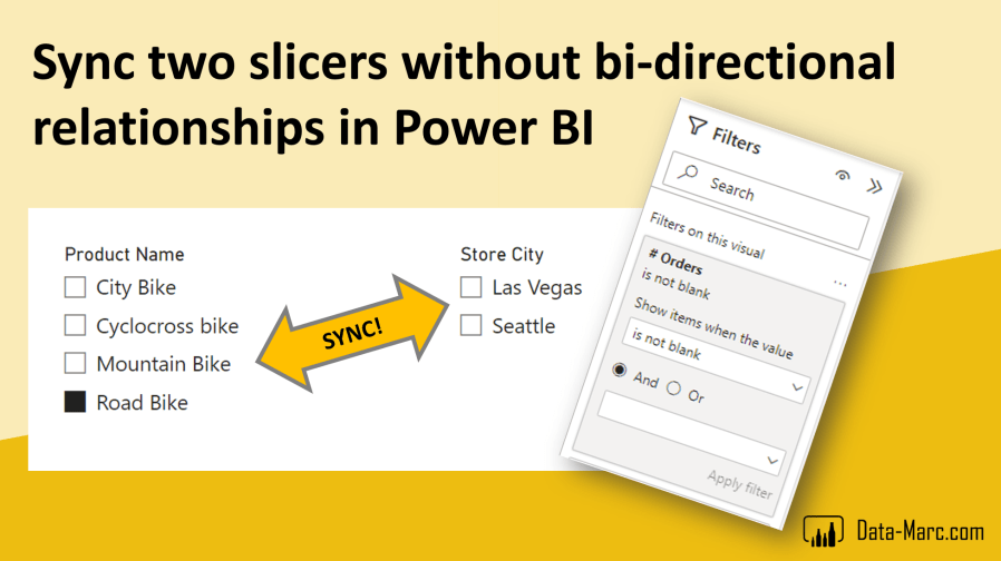
Have you ever wanted to sync two slicers on a report page? Even when both slicers are coming from different dimensions? A lot of users end up setting the relationships to bi-directional (both) which has huge side effects! You may up with a ambiguous data model, over filtering fact tables and wrong results. Also, there is a very likely performance impact to this solution.

But actually, to make the slicers sync, you don’t have to change the relationships! In this blog I will show you how you can sync two (or more) slicers on a report page without changing the relationships or the semantic model!

Intro

Last week, I attended Power BI Next Step conference in Denmark. Always a great occasion to connect with the community, learn and get inspired. For me, it was the fourth time speaking at this conference over the course of four years. Somewhere midday, someone walked up to me and asked if I could explain once again the trick I showed a few years ago to make two slicers sync in a Power BI report. It’s a trick that I showed as part of a data modeling session back then. After showing it once again, I thought, why not directly convert it into a blog? Maybe for you a walk in the park, for others who are starting their Power BI journey it could be a useful tip.

TL;DR Sample file at the bottom!

Set the scene

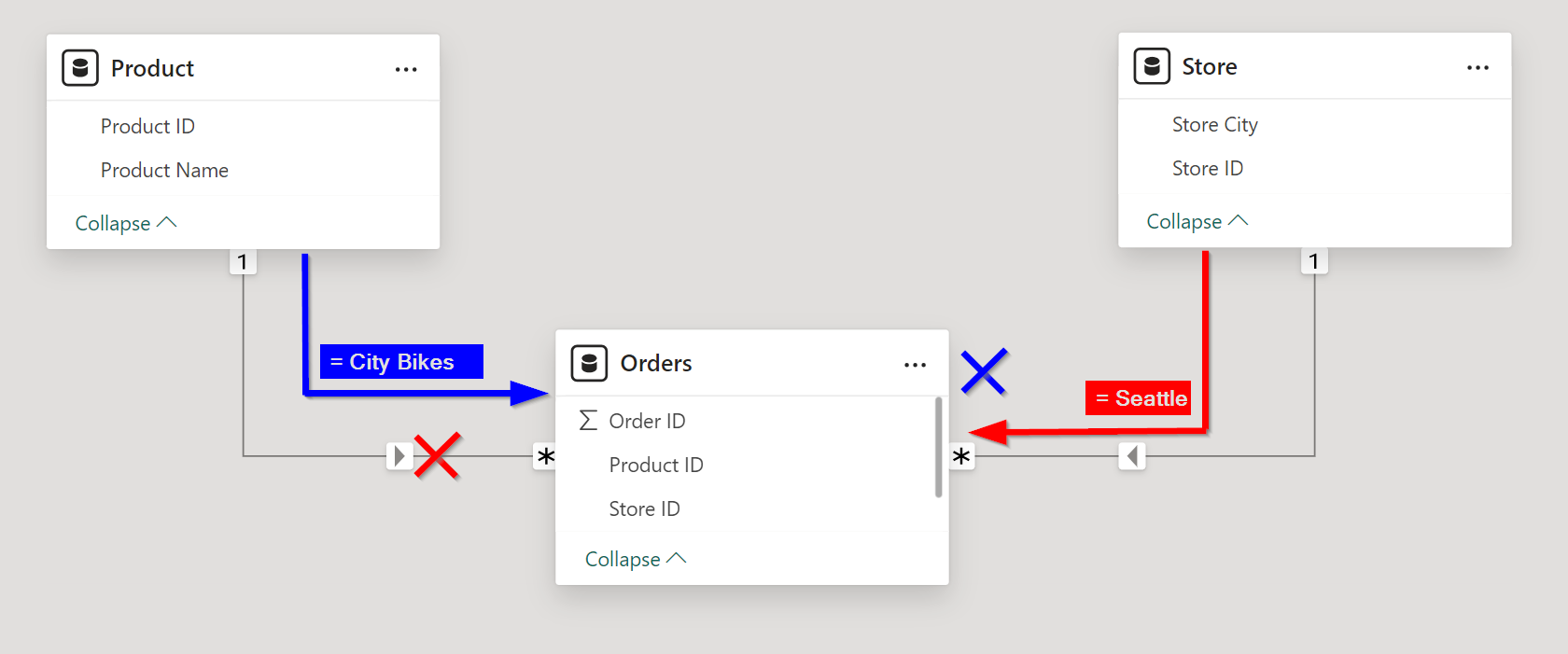
To explain the concept, I setup a very simplified semantic model. In this setup, I have two dimension tables and a fact table that connects them. The dimensions are Product and Store, where the Orders table connects them. All tables in this example are simplified and limited to a minimal set of columns.

As you can see in above example semantic model, both relationships are currently set as 1-to-Many and single direction. This is in line with data modeling best practices. The total set of data exists of 5 products, 5 stores and 10 orders (each order is one row).

Case

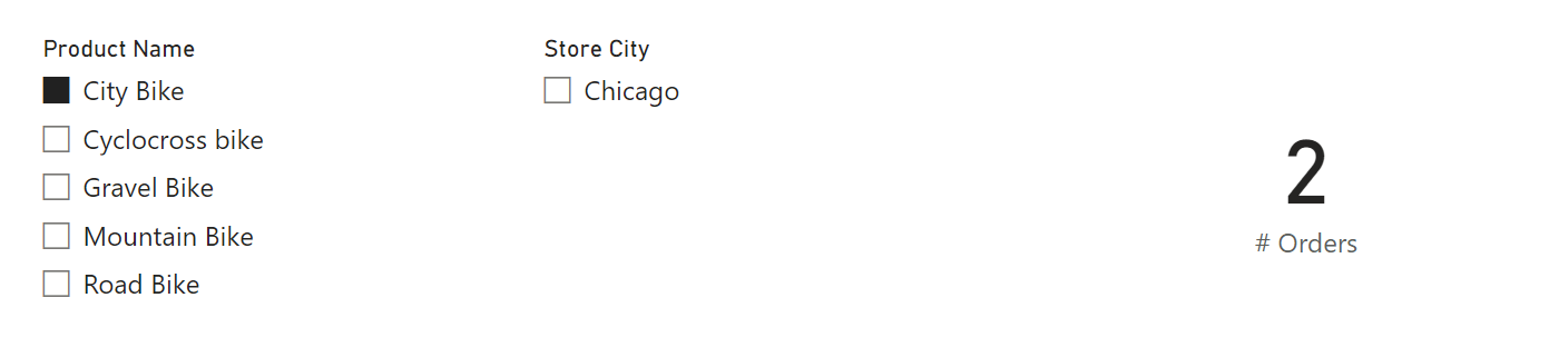
Now, I want to build a report where I have two slicers on the screen, each coming from one dimension. Also, I have a simple count of orders visualized on the screen in a card visual. Intention was not to put together a fancy report, so excuse me for the minimalistic report.

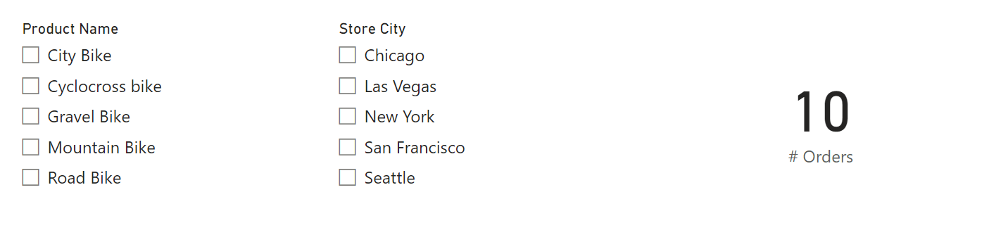
Imagine, I want to make use of both slicers at the same time. Basically, as soon as I filter to the Product Name slicer to only show City Bikes, I only want to see the relevant stores which have ever sold a City Bike.

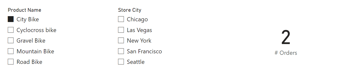
But maybe, at the same time, I want to filter Store City slicer to only look at Seattle, however this leads to the result (Blank) in the # Orders card visual cause we never sold any City Bikes in Seattle apparently.

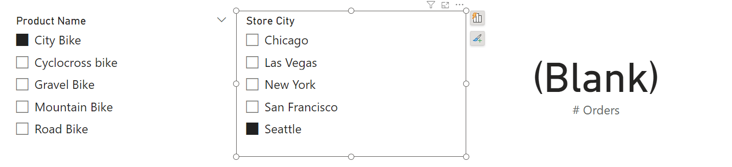
If both slicers would have synced beforehand, I would have seen directly that the combination City Bike and Seattle was not a valid combination for any of the sales orders.

Why it doesn’t work

By default, the expected filter behavior will not work. This has nothing to do with the is due to the interactions between both visuals. The Edit interactions option where you can switch between cross-filtering and highlighting will not help you here. The behavior has everything to do the relationship direction. Looking back at the semantic model, we can see by the filter direction (small arrows), that both dimensions will filter the fact table, but the filter from one dimension will never reach the other dimension.

Doing it the wrong way…

A potential solution you may consider, is to put one, or both relationships to bi-directional (both) cross-filter direction. You can do this in the Edit relationship dialog. Let’s just do this for a second and see if this achieves our result.

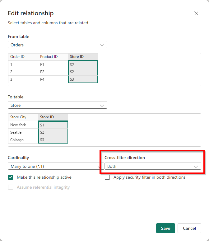
Going back to the report, if I now filter on City Bikes, I can directly see this option is only relevant for the Store City Chicago.

So far, so good, right? Mission accomplished and it does exactly what you want it to do. However, setting relationships to filter in both directions has big side-effects and I would strictly recommend not doing this! There could be valid reasons to do this, but then please be very much aware of what you are doing.

Why you shouldn’t do this!

Having bi-directional relationships in your semantic model does not only have a huge performance impact but can also lead to ambiguous data models. Let’s look closer at the performance impact first.

In the simplified semantic model, used for this blog, with a very minimal set of rows it is almost impossible to measure the performance impact. But imagine setting relationships to bi-directional in a semantic model with multi-million rows and maybe even large dimensions. Every time you apply a filter to one dimension, this filter expression has to be passed through all other dimension tables. This can easily become a heavy operation on your semantic model.

Even worse is ending up with over-filtering and ending up with unexpected results. When this happens, we can call this an “ambiguous data model”. In order to explain this properly, I will use a slightly more complicated semantic model. Typically, over filtering appears when you work with multiple fact tables in your semantic model.

Above example has two fact tables, being Internet Sales and Product Inventory. Both tables share the same dimensions, being Date and Product. Notice the bi-directional relationship between Internet Sales table and Product.

Now, I want to put a filter on the Date dimension to only show data for the year 2024 for example. As a result, I will filter my Internet Sales as well as the Product Inventory as they both have their own filter path identified by number 1 and 4. So far, so good! But, given the Internet Sales table also has an active bi-directional relationship (number 2) to the Product table, the product table will also be affected by the date filter. As a result, the Product table will be filtered down to only show products that were sold in the year 2024. Given the relationship between Internet Sales and Product is based on Product IDs, it no longer has the context of the year filter.

Now, the over-filtering comes in! Because the Product table, also has a relationship (number 3) directly to the Product Inventory where the filter path defines that the dimension filters the fact table. This relationship is also based on Product IDs and is not aware of the year context. As a result, two filters with a different context will reach the Product Inventory.

• The red line: relationship between Date and Product Inventory as it should be (number 4).
• The blue lines: relationship which changes context due to a bi-directional filter (number 1, 2 and 3).

The result is that the Product Inventory will only show products that were on stock in the year 2024 and also sold in the year 2024. Are you sure this is what you were looking for? The inventory will be an incomplete picture of the total inventory and may lead to wrong decisions.

Why not create a single fact table?

A lot in the above scenario could be prevented by not having multiple fact tables. Often, having multiple fact tables is sub-optimal and you ideally combine them in one. But in some cases, two fact tables cannot be combined in one due to being a different granularity or different type of fact table. In this case, the fact tables cannot be combined. The Internet Sales table is an additive fact, where the total sales can be calculated to take the sum of an individual column. Each new sales order will add a new row to the table. While the Product Inventory is a non-additive fact, where we cannot take a sum of a column to calculate the total inventory. Typically, non-additive measurements cannot be summed, but taking an average could still make sense. Often, non-additives are snapshots of a moment in time of a total set.

How should I make the slicers sync?

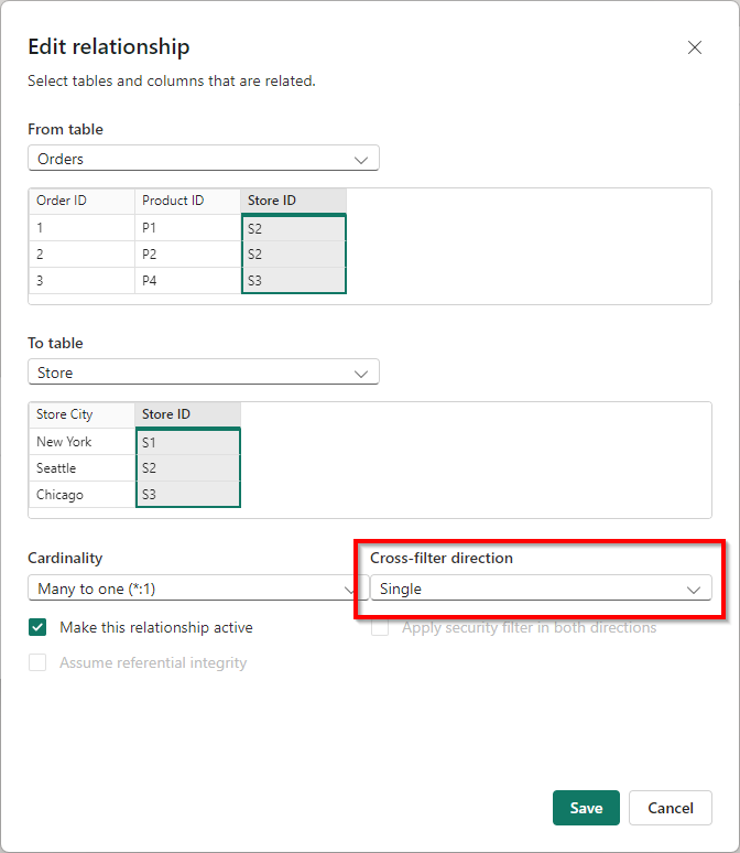
First, we have to make sure we’re back to square one. We remove the bi-directional relationships and have both relationships back to single.

Once we’ve done that for both relationships, we can start defining a simple measure on the fact Table, Orders. We simply want to calculate the count of rows by using the following measure:

# Rows = COUNTROWS( Orders )

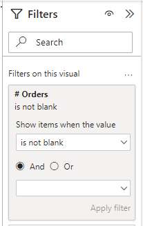
Next, we use this measure as part of a filter on a specific visual using the filter pane. We configure the filter so that the result of # Rows is not blank.

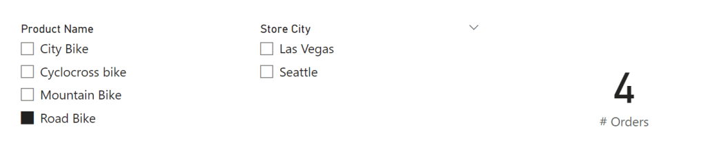
Once, we’ve done that for one slicer, we add the same visual level filter to the other slicer on the screen. A very simple trick which will have the same result as we had before. For example, when we add a filter on Product Name to be Road Bike, we will see only two Store Cities are relevant, being Las Vegas and Seattle.

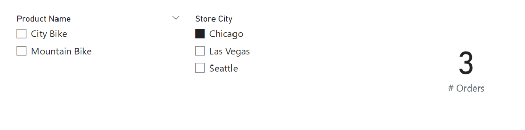
Also, the other way around, if I filter based on a Store City, I can directly see which Product Names are applicable to this Store City. Like in Chicago we only sold City Bike and Mountain Bike.

Considerations

using the measure with a simple countrows instead of changing the relationship direction is a simple and neath solution. However, there are some considerations to take into account. Although, I’m all for this approach, there is one down-side by doing this. In case there is a Store City which has no orders at all, will not show up in the slicer. Therefore, the items presented in the slicer might be an incomplete list of all dimension values available. Depending on your scenario, this may be an issue.

To overcome this, you can consider adding a fake order in the fact table for each dimension value. The behavior of the slicers and corresponding interaction between them remains the same. However, it will pollute your fact table with fake records which you need to flag in some way. For other complex(er) measures you may need to filter out these rows – depending on the exact calculation you aim for. Also, in case of large dimensions and many different dimensions, having a record in the fact table for each possible value will quickly add a lot of rows.

Additional note: Just figured that SQL BI wrote a similar article in 2020. You can find it here.

Sample file

In case you want to go through all the steps above based on the same sample data model, you can download the Power BI file from my GitHub.